
Is corruption influenced by economic growth? Are legal institutions such as the ‘Right to Information Act (RTI) 2005’ in India effective in curbing corruption? Using a panel dataset covering 20 Indian states for the years 2005 and 2008 we estimate the effects of growth and law on corruption. Accounting for endogeneity, omitted fixed factors, and other nationwide changes we find that economic growth reduces overall corruption as well as corruption in banking, land administration, education, electricity, and hospitals. Growth reduces bribes but has little impact on corruption perception. In contrast the RTI Act reduces both corruption experience and corruption perception.
This is a preview of subscription content, log in via an institution to check access.
Price includes VAT (France)
Instant access to the full article PDF.
Rent this article via DeepDyve


Note that Treisman (2000) in Table 1 (p. 411) reports a correlation of 0.87 between Business International and Transparency International macro cross-country data.
Note that Huntington (1968) disagrees with this view. He argues that rapid modernization induces normative confusion at a time when the emerging economic elites are striving for power and influence. As a result growth increases corruption.
Note that the official would never present these objections in writing.Note that the Kolmogorov–Smirnov tests reported in Table 2 indicates that the distribution of corruption across states have changed over the two time periods. Forces such as economic growth may be driving these changes.
More on this in the section ‘Empirical strategy and data’.Ades and Di Tella (1999), Rose-Ackerman (1999), Leite and Weidmann (1999), Dabla-Norris (2000) are other important contributions in this literature. Bardhan (1997) provides an excellent survey of the early contributions.
Note that we also use GDP per capita growth rate in Table 3 and our results are robust.Note that the survey asks some additional questions. However, they are not common over the two time periods in our study. Therefore we are not including them here.
Note that the India Corruption Study only reports these macro percentages and the underlying micro data is not reported.
The model predicts that corruption in Bihar should have declined by 18.5% points due to the RTI Act. However, the actual decline is 30% points. Therefore, the predicted decline is 62% of the actual.
According to our estimates, economic growth reduced corruption perception only in education.We gratefully acknowledge comments by and discussions with Paul Burke, Ranjan Ray, Takashi Kurosaki, Peter Warr, and Conference and seminar participants at the Australian National University, University of Oxford, and ISI Delhi. We thank the editor, Josef Brada, and an anonymous referee for their comments. We also thank Rodrigo Taborda for excellent research assistance. All remaining errors are our own.
Corruption [c it ]: Corruption is computed using a two-step procedure. First, an average is computed of the percentage of respondents answering yes to the questions that they have direct experience of bribing, using a middleman, perception that a department is corrupt, and perception that corruption increased over time for eight different sectors: banking, land administration, police, education, water, Public Distribution System (PDS), electricity, and hospitals. Second, these averages are also averaged over all the eight sectors to generate one observation per state and per time period. Higher value of the corruption measure implies higher corruption. Source: India Corruption Study 2005 and 2008, Transparency International.
Corruption in Banks [c it BANKS ]: Corruption computed in the same fashion as c it but only for the banking sector. Source: India Corruption Study 2005 and 2008, Transparency International.
Corruption in Land Administration [c it LAND ]: Corruption computed in the same fashion as c it but only for the land administration sector. Source: India Corruption Study 2005 and 2008, Transparency International.
Corruption in Police [c it POLICE ]: Corruption computed in the same fashion as c it but only for police. Source: India Corruption Study 2005 and 2008, Transparency International.
Corruption in Education [c it EDUC ]: Corruption computed in the same fashion as c it but only for education sector. Source: India Corruption Study 2005 and 2008, Transparency International.
Corruption in Water [c it WATER ]: Corruption computed in the same fashion as c it but only for the water supply sector. Source: India Corruption Study 2005 and 2008, Transparency International.
Corruption in PDS [c it PDS ]: Corruption computed in the same fashion as c it but only for the public distribution system. Source: India Corruption Study 2005 and 2008, Transparency International.
Corruption in Electricity [c it ELEC ]: Corruption computed in the same fashion as c it but only for the electricity sector. Source: India Corruption Study 2005 and 2008, Transparency International.
Corruption in Hospitals [c it HOSP ]: Corruption computed in the same fashion as c it but only for hospitals. Source: India Corruption Study 2005 and 2008, Transparency International.
Corruption Experience Measures: Corruption experience measures are the average of answers to the questions on ‘direct experience of bribing’ and ‘using influence of a middleman’. Source: India Corruption Study 2005 and 2008, Transparency International.
Corruption Perception Measures: Corruption perception measures are the average of answers to the questions on ‘perception that a department is corrupt’ and ‘perception that corruption has increased’. Source: India Corruption Study 2005 and 2008, Transparency International.
Economic Growth []: Real growth rate in state GDP measured in 2009 constant prices. Source: Planning Commission, Government of India.
Log Rainfall [ln RAIN it−1 ]: Log of rainfall across states measured in millimeters. Source: Compendium of Environmental Statistics, Central Statistical Organisation, Ministry of Statistics and Programme Implementation.
Flood Area: Total area affected by flood in 1994 and 1996 measured in millions of hectares. Source: Central Water Commission, Government of India.
Flood Population: Total population affected by flood in 1994 and 1996 measured in millions. Source: Central Water Commission, Government of India.
Flood Crop Area: Total crop area affected by flood in 1994 and 1996 measured in millions of hectares. Source: Central Water Commission, Government of India.
Flood Household: Total number of households affected by flood in 1994 and 1996 measured in millions of hectares. Source: Central Water Commission, Government of India.
Literacy: Literacy rate for 2002 and 2005. Source: Selected Socioeconomic Statistics India 2006, Central Statistical Organization, Table 3.3.
Gini Coefficient: Gini coefficient urban for the periods 1999–2000 and 2004–2005. Source: Planning Commission.
Poverty Head Count Ratio: Percentage of population below poverty line (rural and urban combined). Source: Planning Commission.
Mining Share of GDP: Mining sector share of state GDP. Source: Handbook of Statistics on the Indian Economy, Reserve Bank of India.
Primary Sector Share of GDP: Primary sector share of state GDP. Source: Handbook of Statistics on the Indian Economy, Reserve Bank of India.
State Government Expenditure: State government expenditure as a proportion of state GDP. Source: Indian Public Finance Statistics, Ministry of Finance.
Newspaper Circulation: Number of registered newspapers in circulation. Source: Registrar of Newspapers, Government of India.
Telephone Exchange: Number of telephone exchanges. Source: Ministry of Information and Broadcasting, Government of India.
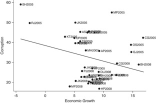
Andhra Pradesh (AP), Assam (AS), Bihar (BH), Chhattisgarh (CG), Delhi (DL), Gujarat (GJ), Haryana (HR), Himachal Pradesh (HP), Jammu and Kashmir (JK), Jharkhand (JH), Karnataka (KT), Kerala (KL), Madhya Pradesh (MP), Maharashtra (MH), Orissa (OS), Punjab (PJ), Rajasthan (RJ), Tamil Nadu (TN), Uttar Pradesh (UP), West Bengal (WB).
Assume that the true relationship between corruption and growth is . However the corruption variable has measurement error so that (where θ it is the time varying measurement error). Because of measurement error we only observe and not true corruption c it . So we estimate the model . While estimating this model using fixed effects we would difference the data and get . The parameter estimate of interest would be, and . Therefore, estimating the model using OLS would yield biased estimates. If we use rainfall instrument Z it that is correlated with but orthogonal (or uncorrelated) to Δθ it , Δβ t and Δɛ it then cov(Z it , Δθ it )=cov(Z it , Δβ t )=cov(Z it , Δɛ it )=0. Then we would get, and since cov(Z it , Δβ t )=cov(Z it , Δɛ it )=0. Therefore, the IV strategy could potentially remedy the measurement error problem with 2008 corruption data.